Isomap for Dimensionality Reduction in Python
Isomap (Isometric Feature Mapping), unlike Principle Component Analysis, is a non-linear feature reduction method.
We will explore the data set used by the original authors of isomap to demonstrate the use of isomap to reduce feature dimensions.
The image below, taken from the original paper by Tenenbaum et al., demonstrates how Isomap operates.
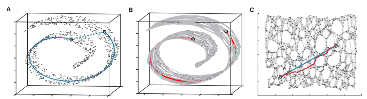
In A we see that two points that are close together in Euclidean Space in this “Swiss roll” dataset may not reflect the intrinsic similarity between these two points.
In B a graph is constructed with each point as n nearest neighbours (K=7 here). The shortest geodesic distance is then calculated by a path finding algorithm such as Djikstra’s Shortest Path.
In C, this is the 2D graph is recovered from applying classical MDS (Multidimensional scaling) to the matrix of graph distances. A straight line has been applied to represent a simpler and cleaner approximation to the true geodesic path shown in A.
Isomap should be used when there is a non-linear mapping between your higher-dimensional data and your lower-dimensional manifold (e.g. data on a sphere).
Isomap is better than linear methods when dealing with almost all types of real image and motion tracking and we will now look at the example that was used in the Tenenbaum et al. of images of faces in different poses and light conditions.
The images are 4096 dimensions (64 pixel x 64 pixel).
We will reduce this down to just 2 dimensions
Scikit-learn isomap
We start by loading our face data.
import math

import pandas as pd
import scipy.io
pd.options.display.max_columns = 7

mat = scipy.io.loadmat('data/face_data.mat')
df = pd.DataFrame(mat['images']).T

num_images, num_pixels = df.shape
pixels_per_dimension = int(math.sqrt(num_pixels))

# Rotate the pictures
for idx in df.index:
    df.loc[idx] = df.loc[idx].values.reshape(pixels_per_dimension, pixels_per_dimension).T.reshape(-1)

# Show first 5 rows
print(df.head())
Now we fit our isomap to our data. Remember that if your data is not on the same scale, it may require scaling before this step.
We will fit a manifold using 6 nearest neighbours and our aim is to reduce down to 2 components.
from sklearn import manifold

iso = manifold.Isomap(n_neighbors=6, n_components=2)
iso.fit(df)
manifold_2Da = iso.transform(df)
manifold_2D = pd.DataFrame(manifold_2Da, columns=['Component 1', 'Component 2'])

# Left with 2 dimensions
manifold_2D.head()
import matplotlib.pyplot as plt
import numpy as np
%matplotlib inline

fig = plt.figure()
fig.set_size_inches(10, 10)
ax = fig.add_subplot(111)
ax.set_title('2D Components from Isomap of Facial Images')
ax.set_xlabel('Component: 1')
ax.set_ylabel('Component: 2')

# Show 40 of the images ont the plot
x_size = (max(manifold_2D['Component 1']) - min(manifold_2D['Component 1'])) * 0.08
y_size = (max(manifold_2D['Component 2']) - min(manifold_2D['Component 2'])) * 0.08
for i in range(40):
    img_num = np.random.randint(0, num_images)
    x0 = manifold_2D.loc[img_num, 'Component 1'] - (x_size / 2.)
    y0 = manifold_2D.loc[img_num, 'Component 2'] - (y_size / 2.)
    x1 = manifold_2D.loc[img_num, 'Component 1'] + (x_size / 2.)
    y1 = manifold_2D.loc[img_num, 'Component 2'] + (y_size / 2.)
    img = df.iloc[img_num,:].values.reshape(pixels_per_dimension, pixels_per_dimension)
    ax.imshow(img, aspect='auto', cmap=plt.cm.gray,
              interpolation='nearest', zorder=100000, extent=(x0, x1, y0, y1))

# Show 2D components plot
ax.scatter(manifold_2D['Component 1'], manifold_2D['Component 2'], marker='.',alpha=0.7)

ax.set_ylabel('Up-Down Pose')
ax.set_xlabel('Right-Left Pose')

plt.show()

We have reduced the dimensions from 4096 dimensions (pixels) to just 2 dimensions.
These 2 dimensions represent the different points of view of the face, from left to right and from bottom to top.