Decision Tree Classifier in Python using Scikit-learn

Decision Trees can be used as classifier or regression models.

A tree structure is constructed that breaks the dataset down into smaller subsets eventually resulting in a prediction. There are decision nodes that partition the data and leaf nodes that give the prediction that can be followed by traversing simple IF..AND..AND….THEN logic down the nodes.

The root node (the first decision node) partitions the data based on the most influential feature partitioning. There are 2 measures for this, Gini Impurity and Entropy.

Entropy

The root node (the first decision node) partitions the data using the feature that provides the most information gain.

Information gain tells us how important a given attribute of the feature vectors is.

It is calculated as:

$\text{Information Gain} = \text{entropy(parent)} – \text{[average entropy(children)]} $

Where entropy is a common measure of target class impurity, given as:

$ Entropy = \Sigma_i – p_i \log_2 p_i $

where i is each of the target classes.

Gini Impurity

Gini Impurity is another measure of impurity and is calculated as follows:

$ Gini = 1 – \Sigma_i p_i^2 $

Gini impurity is computationally faster as it doesn’t require calculating logarithmic functions, though in reality which of the two methods is used rarely makes too much of a difference.

Predicting Survival in the Titanic Data Set

We’ll be using a decision tree to make predictions about the Titanic data set from Kaggle. This data set provides information on the Titanic passengers and can be used to predict whether a passenger survived or not.

In [1]:

import pandas as pd

df = pd.read_csv('data/titanic.csv', index_col='PassengerId')

In [2]:

print(df.head())

             Survived  Pclass  \
PassengerId                     
1                   0       3   
2                   1       1   
3                   1       3   
4                   1       1   
5                   0       3   

                                                          Name     Sex   Age  \
PassengerId                                                                    
1                                      Braund, Mr. Owen Harris    male  22.0   
2            Cumings, Mrs. John Bradley (Florence Briggs Th...  female  38.0   
3                                       Heikkinen, Miss. Laina  female  26.0   
4                 Futrelle, Mrs. Jacques Heath (Lily May Peel)  female  35.0   
5                                     Allen, Mr. William Henry    male  35.0   

             SibSp  Parch            Ticket     Fare Cabin Embarked  
PassengerId                                                          
1                1      0         A/5 21171   7.2500   NaN        S  
2                1      0          PC 17599  71.2833   C85        C  
3                0      0  STON/O2. 3101282   7.9250   NaN        S  
4                1      0            113803  53.1000  C123        S  
5                0      0            373450   8.0500   NaN        S

We will be using Pclass, Sex, Age, SibSp (Siblings aboard), Parch (Parents/children aboard), and Fare to predict whether a passenger survived.

In [3]:

df = df[['Pclass', 'Sex', 'Age', 'SibSp', 'Parch', 'Fare', 'Survived']]

We need to convert ‘Sex’ into an integer value of 0 or 1.

In [4]:

df['Sex'] = df['Sex'].map({'male': 0, 'female': 1})

We will also drop any rows with missing values.

In [5]:

df = df.dropna()

In [6]:

X = df.drop('Survived', axis=1)
y = df['Survived']

In [7]:

from sklearn.model_selection import train_test_split

X_train, X_test, y_train, y_test = train_test_split(X, y, random_state=1)

In [8]:

from sklearn import tree

model = tree.DecisionTreeClassifier()

Let’s take a look at our model’s attributes

In [9]:

model

Out[9]:

DecisionTreeClassifier(class_weight=None, criterion='gini', max_depth=None,
            max_features=None, max_leaf_nodes=None,
            min_impurity_split=1e-07, min_samples_leaf=1,
            min_samples_split=2, min_weight_fraction_leaf=0.0,
            presort=False, random_state=None, splitter='best')

Defining some of the attributes like max_depth, max_leaf_nodes, min_impurity_split, and min_samples_leaf can help prevent overfitting the model to the training data.

First we fit our model using our training data.

In [10]:

model.fit(X_train, y_train)

Out[10]:

DecisionTreeClassifier(class_weight=None, criterion='gini', max_depth=None,
            max_features=None, max_leaf_nodes=None,
            min_impurity_split=1e-07, min_samples_leaf=1,
            min_samples_split=2, min_weight_fraction_leaf=0.0,
            presort=False, random_state=None, splitter='best')

Then we score the predicted output from model on our test data against our ground truth test data.

In [11]:

y_predict = model.predict(X_test)

from sklearn.metrics import accuracy_score

accuracy_score(y_test, y_predict)

Out[11]:

0.83240223463687146

We see an accuracy score of ~83.2%, which is significantly better than 50/50 guessing.

Let’s also take a look at our confusion matrix:

In [12]:

from sklearn.metrics import confusion_matrix

pd.DataFrame(
    confusion_matrix(y_test, y_predict),
    columns=['Predicted Not Survival', 'Predicted Survival'],
    index=['True Not Survival', 'True Survival']
)

Out[12]:

	Predicted Not Survival	Predicted Survival
True Not Survival	98	14
True Survival	16	51

If we have graphviz installed http://www.graphviz.org/, we can export our decision tree so we can explore the decision and leaf nodes.

In [13]:

tree.export_graphviz(model.tree_, out_file='tree.dot', feature_names=X.columns)

We can then convert this dot file to a png file.

In [14]:

from subprocess import call

call(['dot', '-T', 'png', 'tree.dot', '-o', 'tree.png'])

Out[14]:

We can then view our tree, which looks like this (Click to view full):

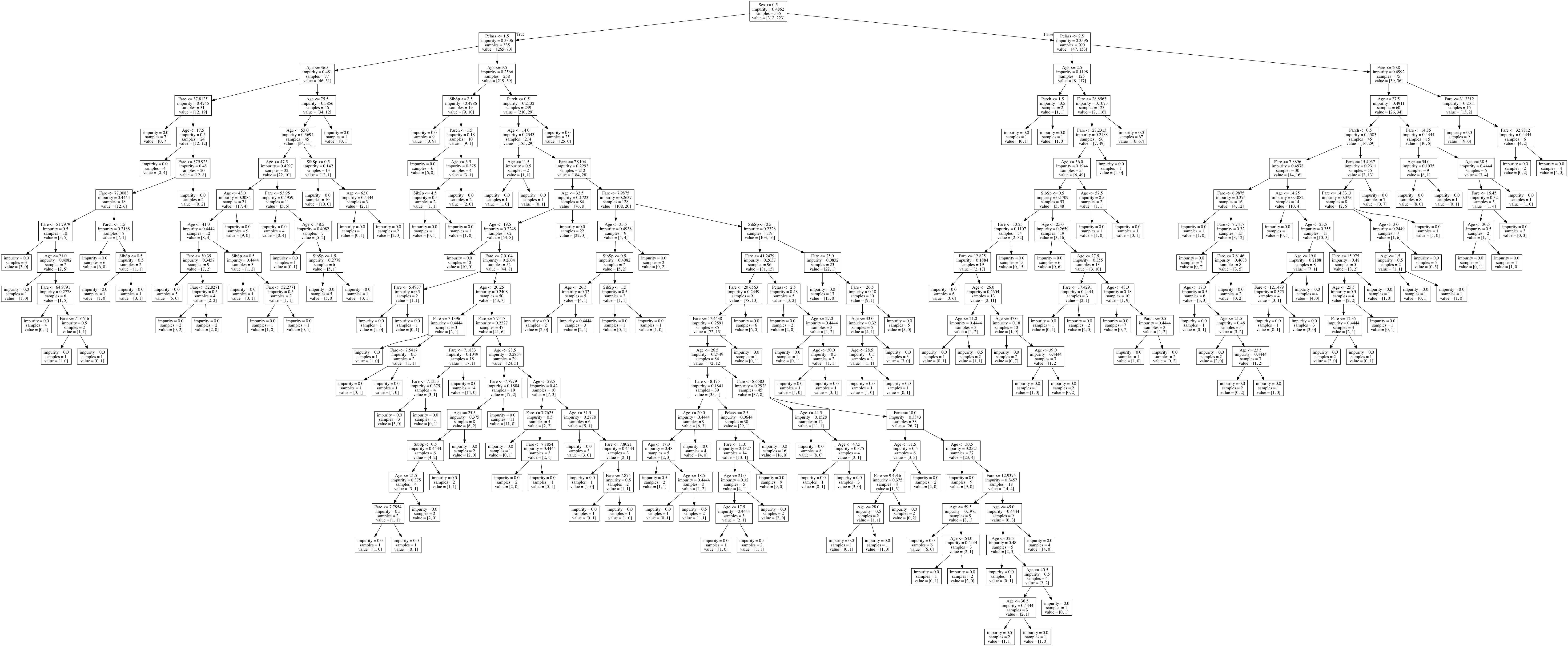
The root node, with the most information gain, tells us that the biggest factor in determining survival is Sex.

If we zoom in on some of the leaf nodes, we can follow some of the decisions down.

We have already zoomed into the part of the decision tree that describes males, with a ticket lower than first class, that are under the age of 10.

'tree_leaf_nodes'

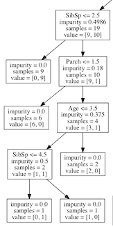
The impurity is the measure as given at the top by Gini, the samples are the number of observations remaining to classify and the value is the how many samples are in class 0 (Did not survive) and how many samples are in class 1 (Survived).

Let’s follow this part of the tree down, the nodes to the left are True and the nodes to the right are False:

We see that we have 19 observations left to classify: 9 did not survive and 10 did.
From this point the most information gain is how many siblings (SibSp) were aboard.
A. 9 out of the 10 samples with less than 2.5 siblings survived.
B. This leaves 10 observations left, 9 did not survive and 1 did.
6 of these children that only had one parent (Parch) aboard did not survive.
None of the children aged > 3.5 survived
Of the 2 remaining children, the one with > 4.5 siblings did not survive.