Support Vector Classifiers in python using scikit-learn

In this post we will be using a Support Vector Classifier (SVC) to classify handwritten digits. This dataset can be found here.

Support Vector Classifiers

SVC aims to draw a straight line between two classes such that the gap between the two classes is as wide as possible.

So we see in the example below we have two classes denoted by violet triangles and orange crosses.

svc-1

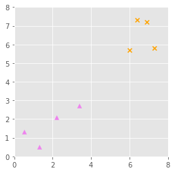
The support vector classifier aims to create a decision line that would class a new observation as a violet triangle below this line and an orange cross above the line.

SVC aims to maximise the gap between the two classes, and we end up with a gap as shown below (red area) and a decision boundary as shown in blue.

svc-2

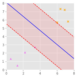
This works fine for examples where the classes can be linearly separated as above.

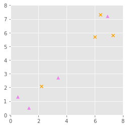
This is rarely the case, often we’ll have something like the case below, where the classes are not linearly separable.

svc-3

In this case, the we would need to transform from this space to another dimension. Kernel functions can provide the dot product of vectors in another space without having to know the transformation into this space. A couple of popular kernels are the ‘linear’ kernel and the ‘rbf’ kernel. We would get a transformation into 3-dimensional space, similar to what’s shown below.

svc-4

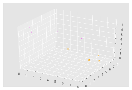
From this, we can now linearly separate the classes as shown by the plane in the graph below.

svc-5

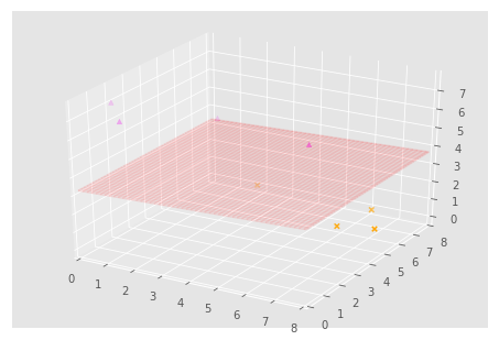
This plane can then transformed to display a non-linear decision boundary in 2-dimensions.

Loading Data

Each row of our data set has 65 columns. The first 64 columns are an 8×8 representation of a grayscale handwritten image. The last column is the label (the number written).

The data comes as a test data file and a training data file, we will load each individually.

In [1]:

import pandas as pd

train = pd.read_csv('data/optdigits.tra', header=None)
test = pd.read_csv('data/optdigits.tes', header=None)

In [2]:

print(train.head())

   0   1   2   3   4   5   6   7   8   9  ...  55  56  57  58  59  60  61  62  \
0   0   1   6  15  12   1   0   0   0   7 ...   0   0   0   6  14   7   1   0   
1   0   0  10  16   6   0   0   0   0   7 ...   0   0   0  10  16  15   3   0   
2   0   0   8  15  16  13   0   0   0   1 ...   0   0   0   9  14   0   0   0   
3   0   0   0   3  11  16   0   0   0   0 ...   0   0   0   0   1  15   2   0   
4   0   0   5  14   4   0   0   0   0   0 ...   0   0   0   4  12  14   7   0   

   63  64  
0   0   0  
1   0   0  
2   0   7  
3   0   4  
4   0   6  

[5 rows x 65 columns]

We now split our data into features and labels:

In [3]:

X_train = train[range(0, 64)]
X_test = test[range(0, 64)]
y_train = train[64]
y_test = test[64]

Let’s have a look at the first 50 numbers, the images and their labels:

In [4]:

import matplotlib.pyplot as plt
%matplotlib inline

idx = 0
for i in range(50):
    plt.subplot(5, 10, idx+1)
    plt.imshow(
        X_train.iloc[idx].values.reshape(8,8),
        cmap=plt.cm.gray_r,
        interpolation='nearest'
    )
    plt.axis('off')
    idx += 1
plt.show()

print(y_train.iloc[0:50].values.reshape(5,10))

[[0 0 7 4 6 2 5 5 0 8]
 [7 1 9 5 3 0 4 7 8 4]
 [7 8 5 9 1 2 0 6 1 8]
 [7 0 7 6 9 1 9 3 9 4]
 [9 2 1 9 9 6 4 3 2 8]]

Creating our Model

We will create an SVC classifier. The SVC classifier comes with a number of tunable parameters.

C is the penalty parameter for the error – A low C value gives a smoother, more generalised decision boundary (high bias) and as you increase C, you increase the variance in your classifier.

Gamma is inversely proportional to the range of the effect of a single training sample – if it is low, the sample will have far-reaching effects, but if it is high the sample will have localised effects only.

The random_state will be set so that we get repeatable results.

It is important to tune these parameters for your model. We will use a C value of 1 and gamma of 0.001 and the radial basis function (rbf) kernel.

In [5]:

from sklearn.svm import SVC

model = SVC(kernel='rbf', C=1, gamma=0.001, random_state=1)

We then train our model on our training data set.

In [6]:

model.fit(X_train, y_train)

Out[6]:

SVC(C=1, cache_size=200, class_weight=None, coef0=0.0,
  decision_function_shape=None, degree=3, gamma=0.001, kernel='rbf',
  max_iter=-1, probability=False, random_state=1, shrinking=True,
  tol=0.001, verbose=False)

We can now score our model on our training data set:

Scoring our model

In [7]:

from sklearn.metrics import accuracy_score

y_predict = model.predict(X_test)
score = accuracy_score(y_test, y_predict)
score

Out[7]:

0.98274902615470228

Our model performs very well on our test set of data and we can visualise this:

In [8]:

idx = 0
fig = plt.figure()
for i in range(50):
    plt.subplot(5, 10, idx+1)
    plt.imshow(
        X_test.iloc[idx].values.reshape(8,8),
        cmap=plt.cm.gray_r,
        interpolation='nearest'
    )
    fontcolor = 'g' if y_test[idx] == y_predict[idx] else 'r'
    plt.title('Predict: %i,\n Actual: %i' % (y_predict[idx], y_test[idx]), fontsize=8, color=fontcolor)
    plt.axis('off')
    idx += 1
fig.set_tight_layout(True)
plt.show()

Looking good.

We can view our confusion matrix to see the most commonly misclassified digits:

In [9]:

import itertools
import numpy as np
from sklearn.metrics import confusion_matrix

cm = confusion_matrix(y_test, y_predict)

classes = range(10)
plt.imshow(cm, interpolation='nearest', cmap=plt.cm.Blues)
plt.title('Confusion Matrix')
plt.colorbar()
tick_marks = np.arange(len(classes))
plt.xticks(tick_marks, classes, rotation=45)
plt.yticks(tick_marks, classes)

thresh = cm.max() / 2.
for i, j in itertools.product(range(cm.shape[0]), range(cm.shape[1])):
    plt.text(j, i, cm[i, j],
             horizontalalignment="center",
             color="white" if cm[i, j] > thresh else "black")

plt.tight_layout()
plt.ylabel('True label')
plt.xlabel('Predicted label')
plt.show()