Deploying Neural Network models to Azure ML Service with Keras and ONNX
In this post we’ll be exploring the deployment of a very simple Keras neural network model to the Azure Machine Learning service using ONNX.
Keras is a high level deep learning library that acts as a wrapper around lower level deep learning libraries such as Tensorflow or CNTK.
We’ll start by locally training a very simple classifier in Keras, serialising this model using ONNX, then deploying this model to Azure ML Service.
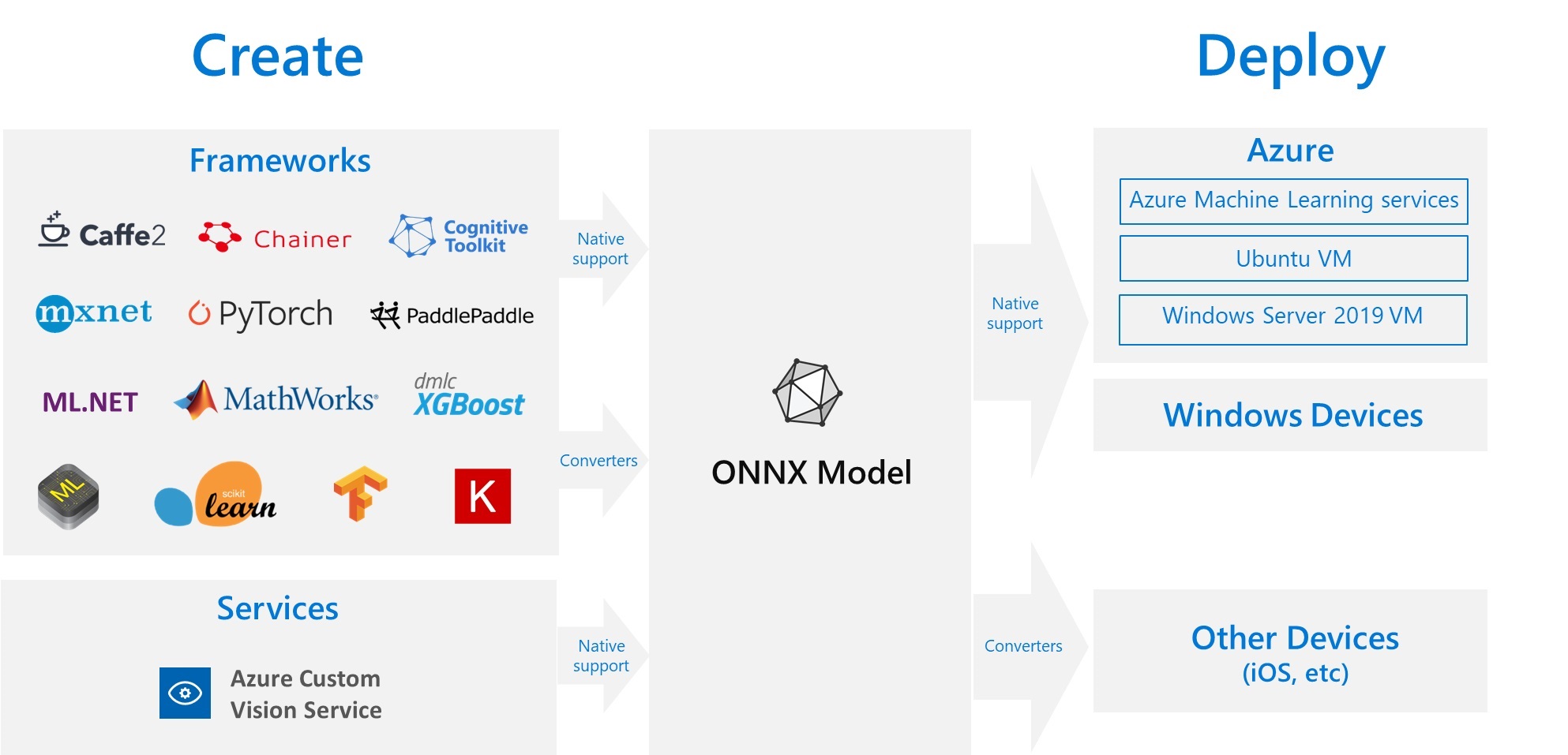
ONNX (Open Neural Network Exchange) is an open format for representing deep learning models and is designed to be cross-platform across deep learning libraries and is supported by Azure ML service.
Quick disclaimer: At the time of writing, I am currently a Microsoft Employee
Training a model
We’ll start by locally training our model in Keras. The model we’ll be using is a very simple model, just a neural network with one hidden layer to categorise handwritten numbers from the MNIST dataset.
In this post I’ll be using Keras with TensorFlow backend. We’ll also need matplotlib to visualise our inputs.
These can be installed by:
pip install tensorflow keras matplotlib
or
pip install tensorflow-gpu keras matplotlib
So let’s start by importing Keras:
import keras
Next we’ll import our training and test data. Keras comes with some functions for loading standard datasets such as the MNIST dataset.
For those that are unaware, the MNIST dataset is a set of handwritten digits that were used for sorting US zip codes in an automated manner.
There is a training set and test set of data.
The training images are a set of 60,000 images of size $28 \times 28$, so the data comes in a 3D array of size $60000 \times 28 \times 28$. The training labels are the numbers 0-9, and this comes in a 1D array of $60000$.
The test images and labels are the same dimensions as the training images and labels but there are only 10,000 observations.
from keras.datasets import mnist

(train_images, train_labels), (test_images, test_labels) = mnist.load_data()
print(train_images.shape)
print(train_labels.shape)
print(test_images.shape)
print(test_labels.shape)
Let’s take a look at the first 10 numbers in the test dataset:
import matplotlib.pyplot as plt

n = 10

fig, ax = plt.subplots(1, n, figsize=(10, 2))
for idx, image in enumerate(train_images[:10]):
    ax[idx].imshow(image, cmap=plt.cm.Greys)
    ax[idx].set_xticks([])
    ax[idx].set_yticks([])
    ax[idx].set_title(train_labels[idx], fontsize=18)

plt.show()
First we flatten our training images such that instead of each input image being $28 \times 28$, we have a single array of $ 784 $ and we normalize the images such that the intensity of each pixel is a number between 0 and 1, rather than 0-255.
# Flatten images
train_images = train_images.reshape((60000, 28 * 28))
# Normalise images
train_images = train_images.astype('float32') / 255

test_images = test_images.reshape((10000, 28 * 28))
test_images = test_images.astype('float32') / 255
For our labels, we’ll want to one-hot encode our labels. These categorical labels are nominal, not ordinal, so there is no concept of the number 6 being “more than” 3 in our categories or vice versa, just as if we were categorising animals, there is no concept of a pig being “more than” a cow.
As such each number will be represented by a 0 (False) or 1 (True) in each position in an array of length 10, with each position representing the digit category of its 0-indexed index in the array i.e. 3 becomes [0, 0, 0, 1, 0, 0, 0, 0, 0, 0].
This can be done using a utility that comes with keras to_categorical.
from keras.utils import to_categorical

train_labels = to_categorical(train_labels)
test_labels = to_categorical(test_labels)
Now we define our neural network architecutre, the input shape is just the flattened shape of our observations, so our input layer has 784 nodes.
We have one intermediate hidden layer with the ReLU (rectified linear unit) activation function, relu as a function is just:
$ ReLU = \max(0, x) $
Our output layer has 10 nodes as output using the Softmax function. The softmax function outputs the probability of a class $j$ given our input vector $x$, $p(j|x)$.
The softmax activation function is calculated as follows:
$ p_j = \dfrac{e^z}{\sum_{j=0}^{9}e^z} $
Where z is calculated as:
$ z = Wa + b $
Where $a$ is the input array from the activation function of the previous layer.
Each number in our output array represents the probability of the label being the category represented by that position in the index:
i.e. [0.01, 0.01, 0.91, 0.01, 0.01, 0.01, 0.01, 0.01, 0.01, 0.01] would represent class 2 being predicted as the most likely output.
The loss function we’ll be using is categorical crossentropy. The categorical crossentropy error is calculated as:
$ Loss_i = -\sum_{j=0}^{9} y_j^i \log{(p_j^i)} $
Where $p_j^i$ is a function of our input sample $x_i$ and our weights and biases to be updated (denoted below as $\theta$).
The total loss is calculated across the samples in our mini-batch $m$.
$Total\ Loss\ (L) = \sum_{i=0}^{m}L_i(\theta;(x^i, y^i)) $
We’ll be using a variant of stochastic gradient descent here that has an adaptive learning rate.
from keras import models
from keras import layers

nn = models.Sequential()
nn.add(layers.Dense(512, activation='relu', input_shape=(28 * 28,)))
nn.add(layers.Dense(10, activation='softmax'))

nn.compile(optimizer='rmsprop',
                loss='categorical_crossentropy',
                metrics=['accuracy'])
With our architecture all set up we’ll now fit our neural network to our training data, we’re going to use a mini-batch size of 128 for our mini-batch stochastic gradient descent and we’ll cover 5 passes of our data.
nn.fit(train_images, train_labels, epochs=5, batch_size=128)
We can then measure our test accuracy by evaluating the neural network model on our unseen test set of data and we can see from our accuracy score that our model performs well enough:
test_loss, test_accuracy = nn.evaluate(test_images, test_labels)

print('test_acc:', test_accuracy)
Serialising Keras model to ONNX format
ONNX (Open Neural Network Exchange) is a format designed by Microsoft and Facebook designed to be an open format to serialise deep learning models to allow better interoperability between models built using different frameworks.
It is supported by Azure Machine Learning service:
ONNX machine learning tools provides us with a method convert_keras for easily converting Keras models to ONNX models. We can then serialise this model to a .onnx file.
These tools can be installed using:
pip install onnxmltools
import onnxmltools

onnx_model = onnxmltools.convert_keras(nn)

onnxmltools.utils.save_model(onnx_model, 'keras_example.onnx')
To test that we can de-serialise run our ONNX model, we’ll use the ONNX Runtime engine, which can be installed by:
pip install onnxruntime
We’ll test whether our model is predicting the expected outputs properly on our first three test images using the ONNX Runtime engine.
We only have one input array and one output array in our neural network architecture.
import onnxruntime

session = onnxruntime.InferenceSession("keras_example.onnx")

first_input_name = session.get_inputs()[0].name
print(first_input_name)

first_output_name = session.get_outputs()[0].name
print(first_output_name)

results = session.run([first_output_name], {first_input_name: test_images[0:3]})

for idx, result in enumerate(results[0]):
    print("Image %d, Actual number = " % idx, test_labels[idx])
    for i, p in enumerate(result):
        print("Probability of %d = %.4f" % (i, p))
Deploy ONNX Model to Azure Machine Learning Service
The steps below are adapted from the Azure Machine Learning service documentation for deploying models to the service.
For this section, we’ll need the Azure Machine Learning service tools installed:
pip install azureml-sdk[notebooks,automl]
We’ll then go through the following steps:
- Create a Machine Learning service workspace
- Register our model with this workspace
- Create a container image for our model
- Deploy this image to Azure ML to create an API for scoring new observations
Creating a Machine Learning service workspace
First off, we create a workspace. This call may be authenticated using your Azure Portal authentication details. The details for this workspace can be serialised to json such that it can then be loaded easily in the future.
If the resource group provided here doesn’t already exist, it will be created. Our resource group is filled with the resources we require for serving our model (e.g. container registry for storing our container image to be deployed etc).
from azureml.core import Workspace

ws = Workspace.create(name='myworkspace',
                   subscription_id='{subscription_id}',
                   resource_group='myresourcegroup',
                   create_resource_group=True,
                   location='westeurope'
                  )
Register our model with this workspace
We then register our ONNX model in this workspace. If we register another model with the same name the version number will be incremented.
from azureml.core.model import Model

model = Model.register(model_path = "keras_example.onnx",
                       model_name = "MyONNXmodel",
                       description = "Test Keras Model",
                       workspace = ws)
Create a container image for our model
After we’ve registered our model, we’ll need to create a container image, this has 3 steps:
- Create a scoring python script file (
score.py) for scoring the new observations that the API is polled with - Create an environment configuration file
- Create an image configuration
- Create container image
We’ll start with the score.py file.
score.py
This script will provide a prediction of classification for new observations that our API will be polled with.
There are two functions, an init function and a run function.
Our init function is called first and will set the path to the model based on the model we registered above.
The run function then does a similar job to when we tested the ONNX model above, it loads the data coming in, casts it to a NumPy array of floats, then loads in the model and gets the results of running our new observations through the model.
The return value is a dict that can be serialised to JSON for returning from the API
%%writefile score.py

import json
import sys

from azureml.core.model import Model
import onnxruntime
import numpy as np

def init():
    global model_path
    model_path = Model.get_model_path(model_name = 'MyONNXmodel')

def run(raw_data):
    try:
        data = json.loads(raw_data)['data']
        data = np.array(data, dtype=np.float32)

        session = onnxruntime.InferenceSession(model_path)
        first_input_name = session.get_inputs()[0].name
        first_output_name = session.get_outputs()[0].name
        result = session.run([first_output_name], {first_input_name: data})
        # NumPy arrays are not JSON serialisable
        result = result[0].tolist()

        return {"result": result}
    except Exception as e:
        result = str(e)
        return {"error": result}
Environment Configuration File
The environment will have a number of external python package dependencies required in order to run the score.py, these are added to our conda dependencies in a yml file we’ve named myenv.yml.
from azureml.core.conda_dependencies import CondaDependencies

myenv = CondaDependencies()
myenv.add_pip_package("numpy")
myenv.add_pip_package("azureml-core")
myenv.add_pip_package("onnxruntime")

with open("myenv.yml","w") as f:
    f.write(myenv.serialize_to_string())
Create an image configuration
We need to provide the configuration for our image so that it knows to run our score.py file using python and requires dependencies in myenv.yml.
This is done by creating an image configuration object:
from azureml.core.image import ContainerImage

image_config = ContainerImage.image_configuration(execution_script = "score.py",
                                                  runtime = "python",
                                                  conda_file = "myenv.yml",
                                                  description = "test"
                                                 )
Create container image
We’re now ready to create our container image. We provide it with the model that we registered, the image configuration we defined above, the workspace we’re working with and the a name.
image = ContainerImage.create(name = "myonnxmodelimage",
                              models = [model],
                              image_config = image_config,
                              workspace = ws)

image.wait_for_creation(show_output = True)
Deploy Image to Azure ML Service
Now that we have our image created, we’ll want to deploy it.
We provide a deployment configuration first with details on the server we’ll deploy our image to – for this example, we’re just going for 1 CPU core and 1 GB of RAM.
We then use the deploy_from_image method to deploy a container from the image we created above.
from azureml.core.webservice import AciWebservice, Webservice

aciconfig = AciWebservice.deploy_configuration(cpu_cores = 1,
                                               memory_gb = 1,
                                               tags = {"data": "mnist", "type": "classification"},
                                               description = 'Handwriting recognition')

service_name = 'keras-mnist-classification'
service = Webservice.deploy_from_image(deployment_config = aciconfig,
                                            image = image,
                                            name = service_name,
                                            workspace = ws)

service.wait_for_deployment(show_output = True)
print(service.state)
print("Scoring API served at: {}".format(service.scoring_uri))
Testing our deployed Azure ML API
We can then poll our API to determine whether we can successfully classify images from our API. The API returns an array of probabilities
There is a service.run method we can use to predict using the deployed model:
import json
import numpy as np
import matplotlib.pyplot as plt

n = 15
sample_indices = np.random.permutation(test_images.shape[0])[0:n]

test_samples = json.dumps({"data": test_images[sample_indices].tolist()})
test_samples = bytes(test_samples, encoding = 'utf8')

# predict using the deployed model
result = service.run(input_data=test_samples)['result']

# compare actual value vs. the predicted values:
plt.figure(figsize = (20, 1))

for i, s in enumerate(sample_indices):
    plt.subplot(1, n, i + 1)
    plt.axhline('')
    plt.axvline('')

    # model returns array of probabilities for each observation, need to select the highest probability class
    predicted_value = result[i].index(max(result[i]))
    actual_value = list(test_labels[s]).index(max(test_labels[s]))
    # use different color for misclassified sample
    font_color = 'red' if actual_value != predicted_value else 'black'
    clr_map = plt.cm.gray if actual_value != predicted_value else plt.cm.Greys

    plt.text(x=10, y =-10, s=predicted_value, fontsize=18, color=font_color)
    plt.imshow(test_images[s].reshape(28, 28), cmap=clr_map)

plt.show()

However, we can also use the URI and make requests using the requests library or using cURL, postman etc. and we can see the outputs are the same as above:
import requests

input_data = json.dumps({"data": test_images[sample_indices].tolist()})

headers = {'Content-Type':'application/json'}

resp = requests.post(service.scoring_uri, input_data, headers=headers)

print("POST to url", service.scoring_uri)

result = json.loads(resp.text)['result']

for i, s in enumerate(sample_indices):
    predicted_value = result[i].index(max(result[i]))
    actual_value = list(test_labels[s]).index(max(test_labels[s]))
    print("{}. Prediction = {}, Actual = {}".format(i, predicted_value, actual_value))
Remember to delete your Resource Group when you’re done.